Excursion in Gleisdreieck Park with Martin

At last, after a record dark start to 2013, Berlin is waking up to bright, clear mornings and the smell and sounds of Spring. Martin and I decided that we would have an excursion together today, after a long gap.

This is the GPS path we made walking around the rather over-designed path layout of the new park.

GPS track from the first exploratory walk of 2013

GPS track from the first exploratory walk of 2013 around Gleisdreieck in Berlin

I decided also to dust off and reassemble my drawing machine. The first two drawings were made with it strapped to the rack of my bike while we walked along pushing it.

Drawing Machine Drawing 1 (On bike, pushing)

Drawing Machine Drawing 1 (On bike, pushing)

Drawing Machine Drawing 2 (On bike, pushing)

Drawing Machine Drawing 2 (On bike, pushing)


This last drawing was made by me carrying it in my hands as I walked. Martin also made a drawing in this way which he kept.
Drawing Machine 3 (Walking)

Drawing Machine 3 (Walking)


On the way back to Bülowstraße, we thought it would be interesting to see what the electromagnetic soundscape was like where the park path takes you near the high-speed track emerging out of the tunnel on the Southbound stretch after Hauptbahnhof. The profusion of overhead power lines tempted us. Luckily I’d brought the coil I’d made from Martin’s instructions on the Psychogeophysics Summit, which I call my Rendlesham Coil.

And this recording was made further on under the bridge where the U2 is turning the corner to head North into Gleisdreieck.

Posted in Diary, GPS, Walking | Tagged , , , , | Comments Off on Excursion in Gleisdreieck Park with Martin

Personal Data Mountain – coding strategies

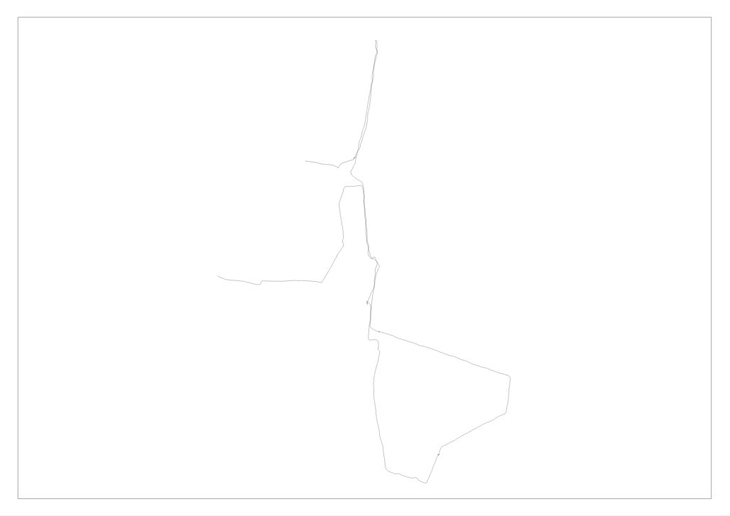
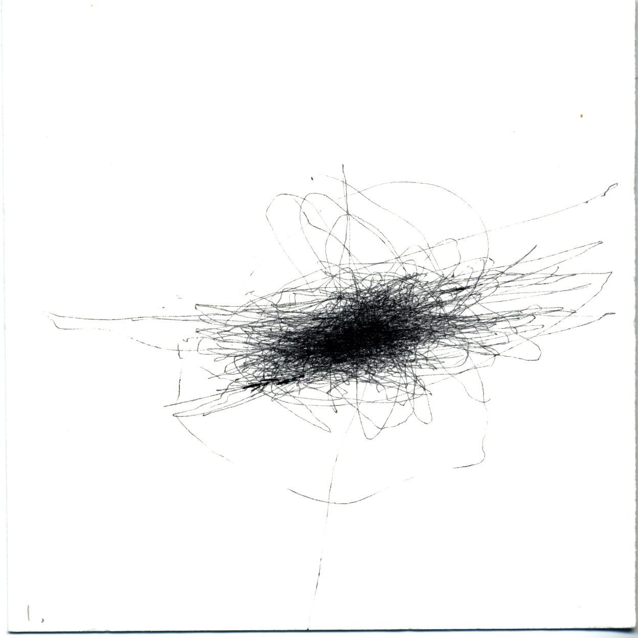
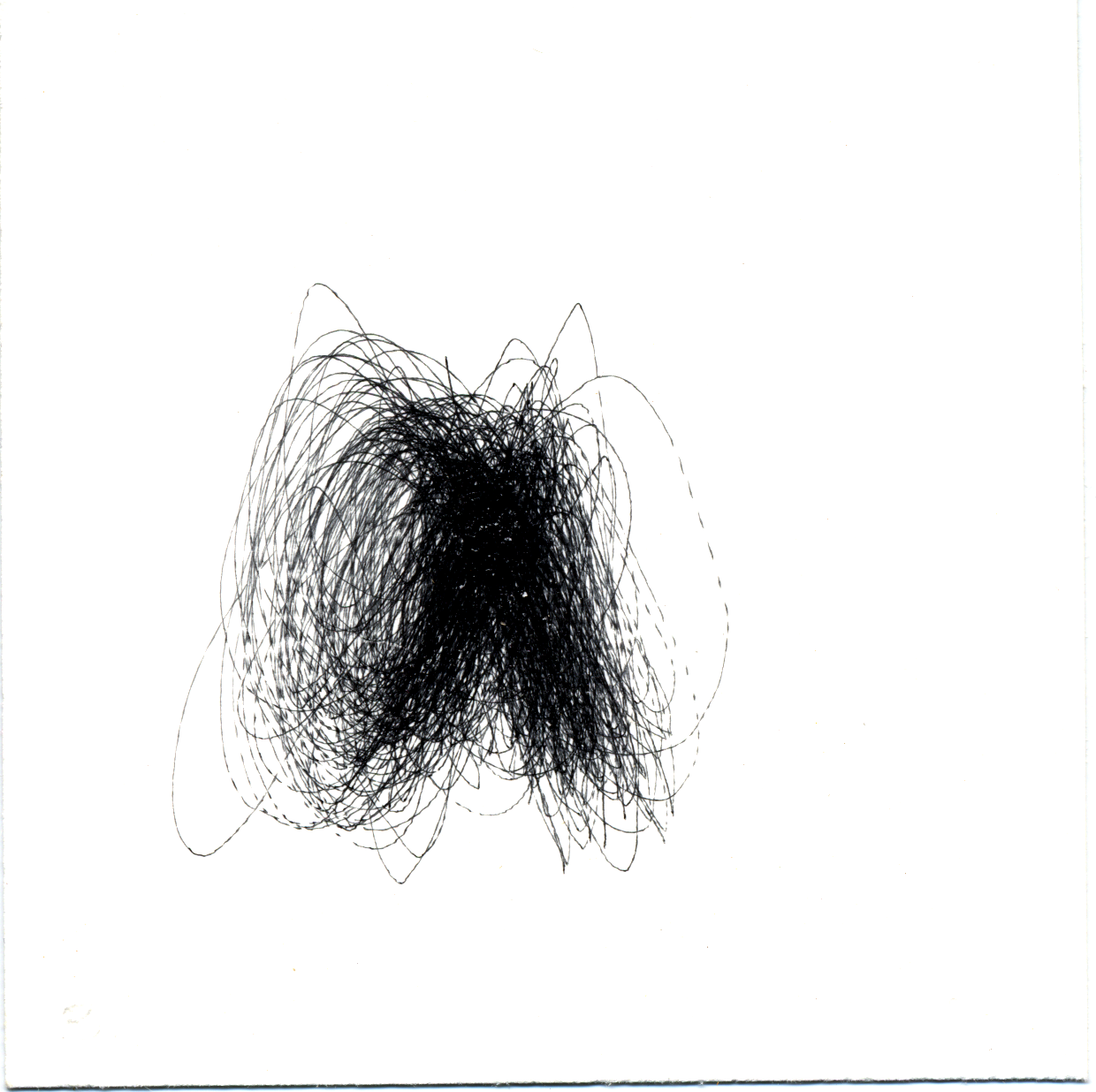
While Soph and I were working last week at the HZT on plan b stuff again at last, we were thinking about the data we collect i.e. GPS, text messages, mood reports (for 2011 only) and photographs.

We were preparing something for the try-out we did last Thursday in which we performed Narrating Our Lines live in front of an invited audience to see if this also worked as a performance, not just a video installation.

One of the things we wanted to try was a fast slideshow (actually a movie) of all the photos we took in the year we decided to play (2007). As I am unsatisfied with any photo management programme I have tried, preferring to order by location rather than date, the photos are scattered among multiple directories.

I knew I could use ffmpeg to stitch individual photos together into a movie, once I’d resized them with the excellent mogrify command in imagemagick, but I needed something that would copy all the photos taken in 2007 to a location so that I could work on them, so I wrote a quick python script you can examine/download below if you’re interested.

#!/usr/bin/env python
# -*- coding: utf-8 -*-

"""
copyimages.py
2013/01/07 19:55:57 Daniel Belasco Rogers dan@planbperformance.net

User points script at a root directory and script finds all images for
a certain year derived from the Exif data and copies these images into
a destination folder supplied by the user

This program is free software: you can redistribute it and/or modify
it under the terms of the GNU General Public License as published by
the Free Software Foundation, either version 3 of the License, or (at
your option) any later version.

This program is distributed in the hope that it will be useful, but
WITHOUT ANY WARRANTY; without even the implied warranty of
MERCHANTABILITY or FITNESS FOR A PARTICULAR PURPOSE.  See the GNU
General Public License for more details.

You should have received a copy of the GNU General Public License
along with this program.  If not, see <https://www.gnu.org/licenses/>
"""

from optparse import OptionParser
from shutil import copy2
import os
import pyexiv2
import sys

def parseargs():
    """
    """
    usage = """
%prog   """
    parser = OptionParser(usage, version="%prog 0.1")
    (options, args) = parser.parse_args()
    if len(args) != 3:
        parser.error("""
Please enter a year in the form YYYY, a directory to search for images
under and a directory to save a copy of the images to
e.g. copyimages.py 2007 "/nfs/photos/" "/media/ext3/"
""")
    year = args[0]
    searchpath = args[1]
    destination = args[2]
    return year, searchpath, destination

def getexifdate(pathname):
    """
    get creation date from exif
    """
    metadata = pyexiv2.ImageMetadata(pathname)
    try:
        metadata.read()
    except IOError:
        print "%s Unknown image type" % pathname
        return False
    try:
        tag = metadata['Exif.Photo.DateTimeOriginal']
    except KeyError:
        print '%s tag not set' % pathname
        return False
    return tag.value

def findimages(year, searchpath):
    """
    ùse os.walk to find images with .jpg extension
    """
    year = int(year)
    imagelist = []
    for (path, dirs, files) in os.walk(searchpath):
        for f in files:
            pathname = os.path.join(path, f)
            if os.path.splitext(pathname)[1].lower() == '.jpg':
                imagedate = getexifdate(pathname)
                if imagedate:
                    try:
                        imageyear = imagedate.year
                    except AttributeError:
                        print '%s invalid date in exif: %s' % (pathname, imagedate)
                        continue
                    if imageyear == year:
                        imagelist.append(pathname)
    return imagelist

def copyimages(imagelist, destination):
    """
    iterate through imagelist, copying images to destination directory
    make the dir in a different way by checking if it is present first
    and making it if not, rather than catching it like this.
    """
    for image in imagelist:
        destinationpath = os.path.join(destination, os.path.split(image)[1])
        print "copying %s to %s" % (image, destinationpath)
        # try:
        copy2(image, destinationpath)
        # except IOError:
        #     os.mkdir(destination)
        #     copy2(image, destination)
        # except OSError as e:
        #     print e
        #     sys.exit(2)
    return

def main():
    """
    call all functions within script and print stuff to stdout for
    feedback
    """
    year, searchpath, destination = parseargs()

    print "Looking in %s for images from %s" % (searchpath, year)
    imagelist = findimages(year, searchpath)
    print "Found %d images" % len(imagelist)

    print "Copying images to %s" % destination
    copyimages(imagelist, destination)
    print "Copied %d images. Script ends here." % len(imagelist)

if __name__ == '__main__':
    sys.exit(main())

All this made me think, however, how much we are all becoming used to this idea of having too much data to sort through. I think its something that lots of us can now relate to when it comes to digital photographs. Running the script above I found about 2500 photos, representing gigabytes of data. Some of the photos I hadn’t seen since I took them and were gathering digital dust somewhere in a remote corner of my filing un-system. To make this stuff (our stuff) understandable, or even viewable, graspable, we need tools to manage it. It is no longer possible or even appropriate to browse through our photos and pull out the ones we’re interested in, we need tools to do this for us.

I have to admit to a feeling of great pride and joy that I could write my own, thanks to acquiring some basic Python skills over the past couple of years.

Posted in Code, Diary, Python, Software | Tagged , , | Comments Off on Personal Data Mountain – coding strategies

The problems with representing GPX tracks in spatial databases

This is something I’ve been wrestling with for a while, both with Spatialite and latterly with Postgis. The problems stem from the fact that a GPX track segment contains information that can be represented in two entirely different ways in these systems. A track segment as represented in a GPX file, as we know contains track points that each have attributes like latitude, longitude, elevation and time and can have more such as speed and course (both of these are calculated between the current point and the previous one). You can import these points into a spatial database (most straightforwardly through an intermediary like shape files), but the devil is in the details and it might surprise you if like me you are used to programmes that have been written to handle GPX files and visualise these rather than larger GIS applications.

The crux is – if you want to see your tracks as lines, you lose the information that each track contained and are left with the segment represented as a row in the database – if you want to retain all the information, you’d better import those trackpoints as points, but then you don’t have a graphical representation of the line each segment represents. Perhaps a couple of illustrations will elucidate the problem

gpx file represented as points

gpx file represented as points in Qgis

Here you see what happens when you import a GPX file into Quantum GIS as track points. This is how it would then be imported into a spatial database. The advantage here is that if you open up the attributes of the file, all the information from the original file is there. I don’t know about you however, but I find it quite difficult to trace the individual track segments from these points – you have an idea of where the road is but no idea about how many times the street is reiterated.

gpx file represented as lines in Qgis

gpx file represented as lines in Qgis

This is more like it – but is it? If you looked at the information each line contains, you’ll see that all the information about the individual points is lost – each line is represented by a single row in the attributes data and so information about the elevation, speed, time of each track point has been lost. Better not use this as a way of archiving your GPS data.

At the moment, other than designing your own database schema and writing your own importers (which is what I’m contemplating), there’s no way I know of in the spatial database world of representing a GPX file in one instance that retains its lines and the information about each point. Please prove me wrong.

Posted in Diary, GPS, Software | Tagged , , , , , , , | 1 Comment

My Life as a Birch Forest

GPS activity charts 2004 - 2011

GPS activity charts 2004 – 2011

The image above is from the Jacquard Loom series (see here and here), using my python script to read a year’s worth of data from our GPS records and plugging in Peter’s processing script, the strips were produced, showing GPS activity much as in the previous posts.

The birch forest is ordered in the following way: the first strip on the left is 2004 (I started recording all my movements in April 2003 but have left this first incomplete year out of this for the moment), each strip being a year ending at 2011 on the right. January is top and December bottom, each black block is a half-hour period in which I recorded some GPS trace. The left of each ‘trunk’ is midnight.

Trips across the planet to other time zones show up as disruption to the blank strip on the left i.e. I appear to be active during the early hours of the morning as the GPS keeps recording time at UTC (or roughly speaking, GMT). The odd dot on the left are late-night outings that get less frequent after 2005 and the birth of our daughter.

The blank strips that go left to right are failures of data collection of some sort: forgetting to download, missing cable while away, lack of batteries etc.

Posted in Code, Diary, GPS, Linux, Python, Software | Tagged , , , , | Comments Off on My Life as a Birch Forest

Jacquard Loom GPS visualisation II

Processing Jacquard Loom Visualisation

Processing Jacquard Loom Visualisation January 2012

After meeting up with Peter at Martin’s micro_blackdeath ATmega noise workshop at NK on Saturday, we were able to talk a bit more about what I’m calling the Jacquard Loom GPS visualisation of the activity in our database.

The python script wot I wrote a while ago visualises a 24-hour period as a line of text, the column width of which you can determine. If there is a GPS recording in the period in question, an asterisk is inserted, otherwise a space is shown. This gives a visual impression of how much (or how little) data we actually record each day.

The earlier post shows the output of this script as a printout from a dot matrix printer but I was talking to Peter about a processing application that reads the script output of asterisks and spaces and visualises this as simple black boxes and gaps. Even though he has plenty to do to finish his MA, he whipped up a quick script that produced the image above.

The picture above shows 1 month (January 2011 – there are 31 lines), the black is where there is GPS data, the white where there is none. The blank space in the left of the image is the time from midnight, so basically no GPS because we’re asleep or at least at home. Because there are 48 blocks, each block represents 30 mins. Compare the image above from Winter to this one below from Summer where you can clearly see the effects of the warmer weather and how it effects our GPS data.

I’d still like to see this knitted…

Processing Jacquard Loom Visualisation June 2012

Processing Jacquard Loom Visualisation June 2012

Posted in Diary, GPS, Linux, Python, Software, Ubuntu | Tagged | Comments Off on Jacquard Loom GPS visualisation II